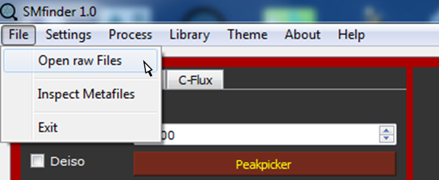
From File, select Open raw Files

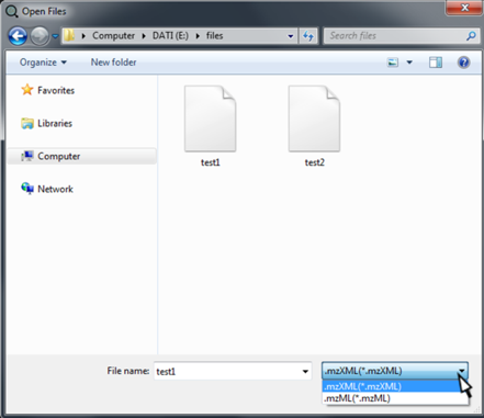
In the new opened window browse the files you want to analyze. Files can be in mzXML or mzML format. By clicking on Open, the "Open Files" dialog, the file are uploaded into SMfinder.

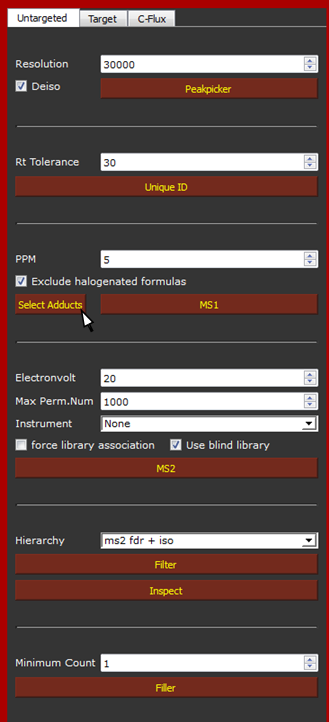
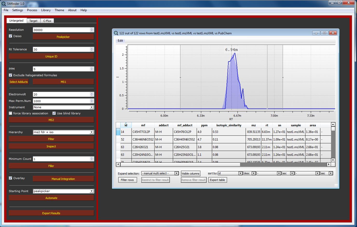
We can now define the parameters for the analysis as it showed below. For further detail on each parameter and button please read the User Guide.

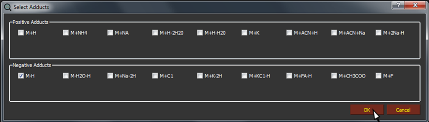
By clicking on Select adducts, a popup will appear. Only the selected types of adducts will be used for analysis. Multiple choices are allowed, while if no adducts are selected the software will used "M+H" for positive and "M-H" for negative mode as default adducts.

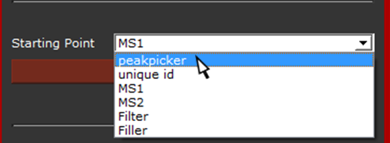
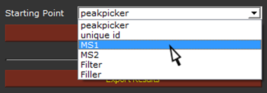
After setting peakpicker as starting point the analysis can be run automatically using the "Automate" button. As alternative option, the analysis can be performed step-by-step keeping in mind that all the processes need to be run in the same order as appear in the Starting point list, with the exception of "Filler" which is an optional function.

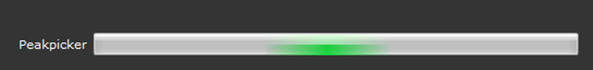
After clicking on Automate or on a specific process, a waiting bar will appear, displaying the running operation.

At the end of the analysis, the waiting bar will disappear, and data will be ready to be explored or exported.
Analysis time can last from minutes to hours depending on computer performance and file complexity.

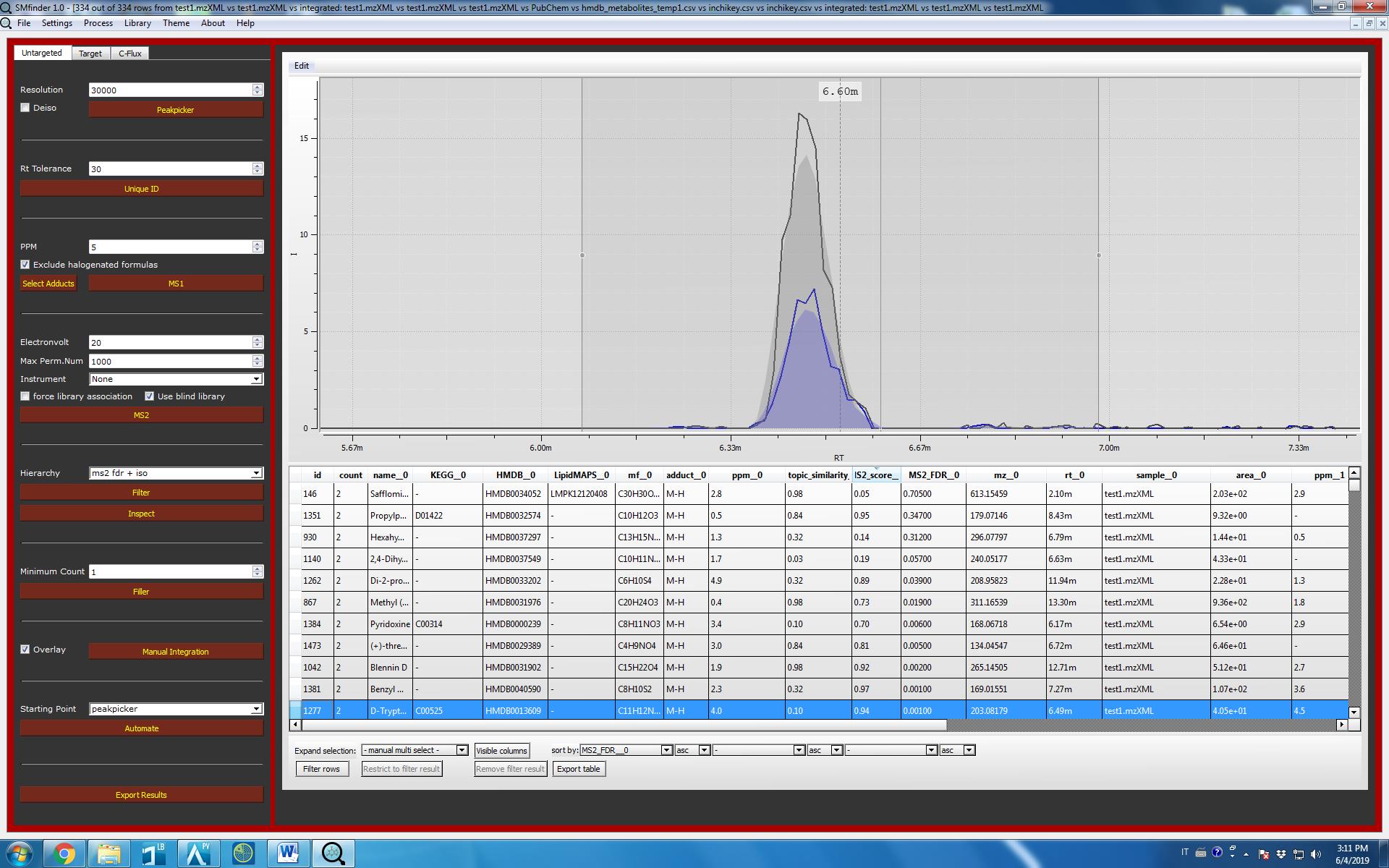
We can explore the result by clicking on “Inspect” button. A table will appear on the central SMfinder box. If you used our test files, you should find 334 detected features. Now we can sort by MS2_FDR__0 which correspond to the FDR of the first file, while MS_FDR__1 correspond to the second selected files etc. etc. We can further filter the name of columns we want to visualize in our output by clicking on “Visible Columns”. Now your output should be similar to the screenshot displayed below.

Now you can export results simply by clicking on Export table. In this case, an Excel file with the information of all the columns will be created.

As alternative, you can used "Export Results" button.

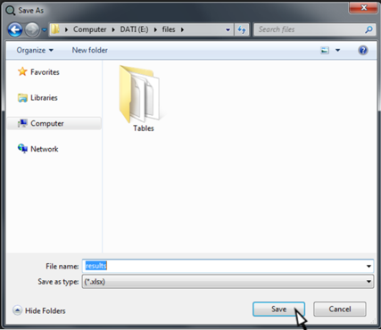
A new windows dialog will ask to save the current results as excel file (.xlsx).

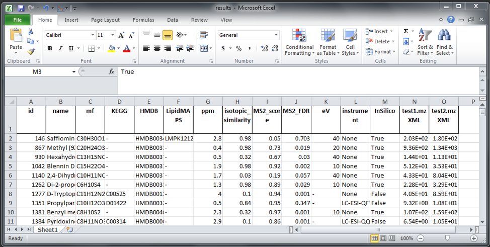
This option will extract core informations such as assigned ID, name, molecular formula (mf), KEGG, HMDB and LipipdMAPS ids. Moreover, the best match for the four identification parameter i.e. ppm, isotopic similarity, MS2 score, MS2 FDR will be reported. eV, Instrument and InSilico are information derived from the library indicating which was the collision energy that give the best match with the idenfied compound, the relative instrument name by which the MS2 spectra was generated and if the spectra is InSilico (True) or empirically acquired (False). Following columns will report the file name in the title and contain the area of detected compounds.

If we want to re-process the dataset without restarting from the beginning, we can do so by modifying the software parameters. As examples, we may want to change PPM, and restart the analysis from MS1 in automatic mode, or change the number of permutations (Max. Perm. Num.) and re-evaluate the samples from MS2. This option shorten the time required to re-analyze the samples.

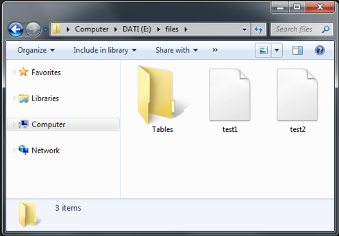
After analyzing a sample or a batch of samples, a new folder named "Tables" will appear in the original folder containing the chromatograms. In this folder, SMfinder will store all the metadata generated by each function as ".table" files.

All metadata are fully explorable by selecting "Inspect Metafiles".

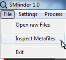
By clicking on "Inspect Metafiles", a new dialog window will open. Now we can select and open the metafile we want to inspect. Notably, this option does not allow the modification of metafiles, but only the inspection.

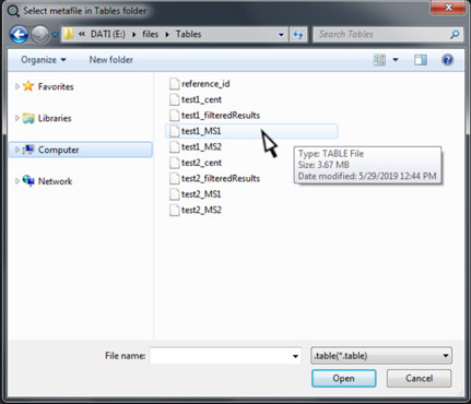
After clicking on "Open", the metadata will appear in the central window of SMfinder.

This workflow can be used to retrieve MS² spectra validated chromatograms e.g. were standards were acquired and stored as chromatograms in public repositories, or from in-house acquired chromatograms.

Start by selecting Target tab in the tab.

We have to create now a reference table for targeted analysis i.e. the compounds we want to identify. Click on "Generate".

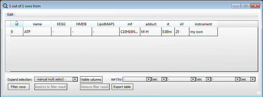
A new table will appear in the central box of SMfinder. Now we can edit the table by inserting the information of the first compound we want to identify.

Moving the mouse on the left side of the row, right-click and select "Clone row".

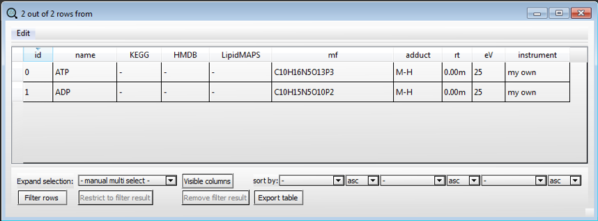
A new row will appear and can be edited with the information of the second compound we want to identify and so on for the entire list of compounds in our target analysis.

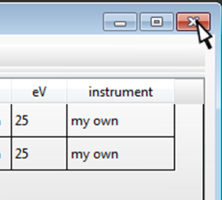
We can now close the generated list by clicking on the red X on the top-right corner of the dialog window.

After closing a new dialog will open asking to save the newly generated reference table.

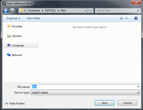
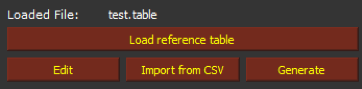
After "Save", if no errors occurs e.g. unknown adduct format inserted, typos in the molecular formula etc., the name of the reference table will appear close to "Loaded File:".

The table can be edited at any time by clicking on Edit button. After editing, closing the tab will overwrite the original table.

We can now select the files in which we want to extract MS2 spectra. As for untargeted analysis, we have to select Open raw files from File in the menu.

Now if we are not sure about the retention time of the compounds, we can check the extracted ion chromatograms by clicking on "Check retention time". If a list of samples is selected, only the first chromatogram of the list will be displayed for retention time evaluation.

We can edit the retention time values and close the window to save.

We are now ready to run target analysis.

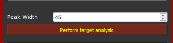
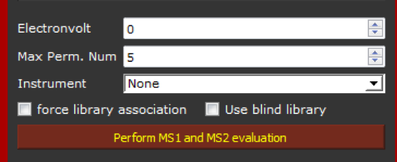
We can now click on "Perform MS1 and MS2 evaluation". In this case, this option is not required to validate the identification, but simply to extract MS² spectra if any, from the selected peaks. In order to speed-up the extraction, we recommend set the number of permutation at 5 (the minimum allowed value) as it is showed below.

Warnings: when modifying retention time or reference table or by using "Inspect metafiles" while other processes are running, it may occur the following error message "Error: one or more previous steps needed". In that case, if previous steps have been all correctly performed, restart SMfinder, reload the reference table and raw files and restart "Perform MS1 and MS2 evaluation".

At the end of the process, the waiting bar of "Perform MS1 and MS2 evaluation" will disappear.

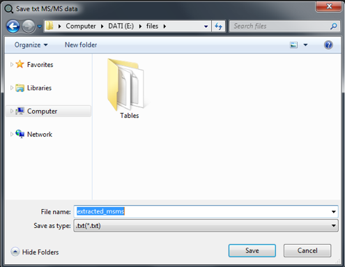
We can now click on "Export txt for library" button.

A new dialog window will appear and allows the save of the spectra in .txt format.

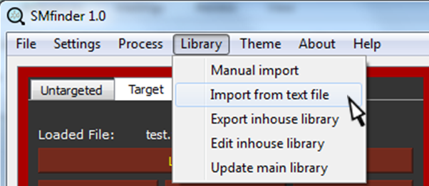
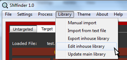
We are now ready to import the MS² spectra into our library. In the menu, under Library tab, select "Import from text file".

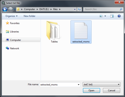
Select the txt file in the dialog window and click on "Open".

The dialog will close and the MS² spectra will be added into SMfinder library.

The correct insertion can be verified by selecting Edit inhouse library under Library tab.

After clicking, the library will open in the central SMfinder box and displays the compounds imported from the selected txt file.

Now that the library has been enlarged, we can use to increase the identification coverage also in previously acquired dataset without the need of re-computing the entire analysis (see the last step in Example of untargeted analysis pipeline).

The C-Flux module allows the analysis of the isotopologues of each compound and it is suitable for 13C labelling analysis.

We start this analysis by creating a reference table for the C-flux module.

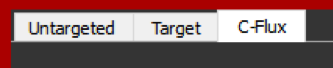
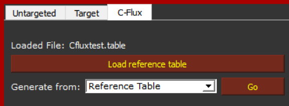
First, we need to click the C-flux tab

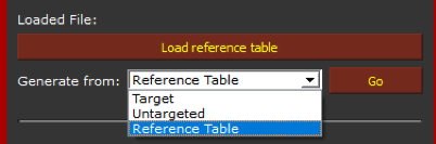
Following, in the "Generate from:" window select Reference table and click on "Go".

This action will open a new dialog window.

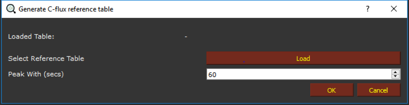
By clicking on Load, we can upload a reference table e.g. the test.table generated in “Using targeted analysis to expand the MS2 library”. After clicking on “OK”, all the masses of potential isotopologues will be automatically calculated and a new dialog will open asking to save the table.

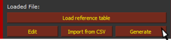
Now we can load the newly generated table by clicking on “Load reference table”. If the table is correctly loaded, it will appear next to the “Loaded File” as it is showed below.

We can now load the raw files we want to analyze by clicking on "Open raw files" in the File menu.

We can now start the analysis by clicking on "Mine 13C Loading".

A waiting bar will appear while the analysis is performed, and disappear at the end of the process.

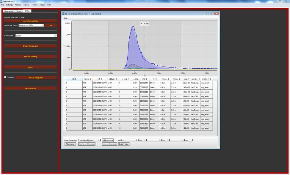
We can now inspect the file using the “inspect” button. We can still use our test files for check the results. Although, those files are not generate for 13C tracing analysis, we can still observe the natural isotopic distribution. As it is showed in the example below, two new columns appear on the table compare with target analysis: “n_carb” and “loading”. These two columns represent respectively the number of labelled carbon that composes the isotopologue and the loading which represent the relative abundance of each isotopologue.

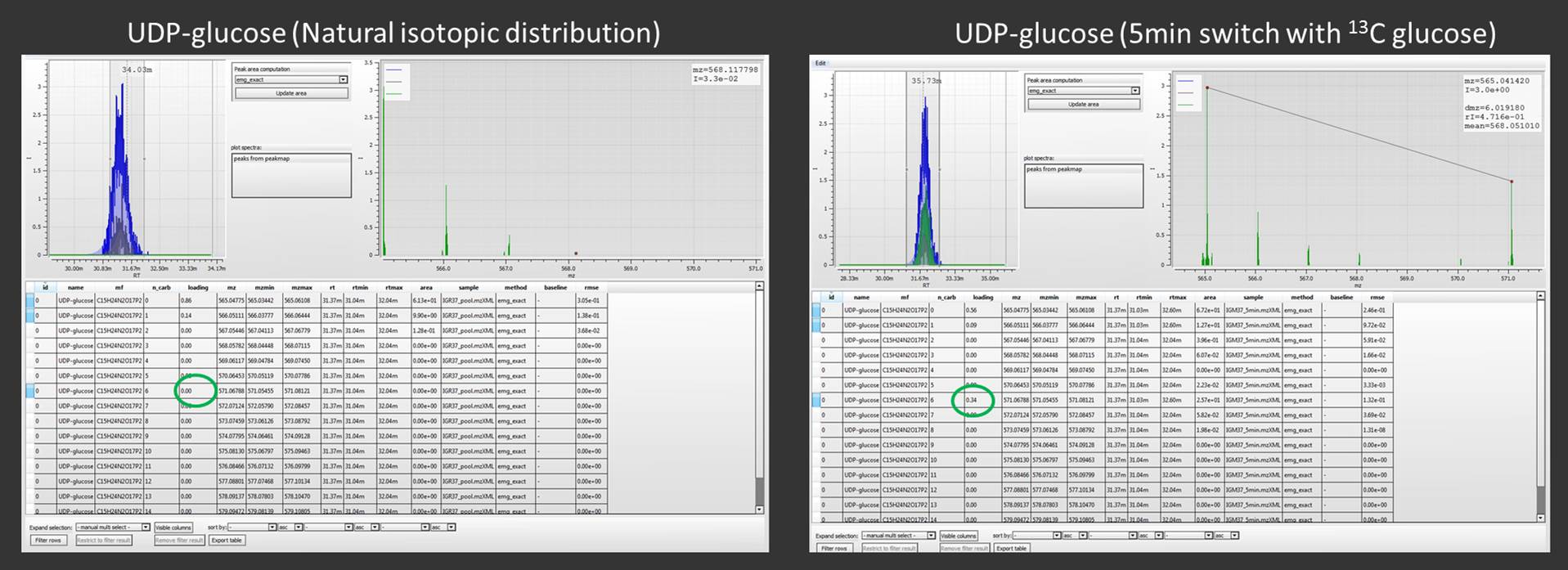
Using a real example, we compared 2 chromatograms from cells without 13C glucose and cells were the glucose was switched to 13C glucose for 5 minutes. By analyzing the isotopic distribution of UDP-glucose we found that the first sample contains only UDP-glucose with a natural isotopic distribution, while in the chromatogram were from the glucose switch experiment, we can observe the isotopologue M+6 which to represent the 34% (green peak) of the total isotopological amount of UPD-glucose.

Finally, we can export the results as an excel file which will report the percentage of loading for each isotopologue.